Characteristics of STARs in Florida
STARs are workers who are “Skilled Through Alternative Routes”. This population of the workforce comprises of working aged adults who have not attained anything educationally past a High School Diploma, yet, have demonstrated the ability to hone their skill to a competitive edge in the labor market.
Usually, STARs go through military service, community college, training programs, partial college completion, or, most commonly, on-the-job experience. STARs can be found in every sector of the workforce, from retail, travel, and hospitality to health care, information technology, manufacturing, and more. (source: https://www.tearthepaperceiling.org/about-stars)
For the purposes of this analysis, I will only be focusing on STAR presence in the state of Florida.
Setup
#Load libraries

library(tidyverse)
library(ggrepel)
library(scales)
library(knitr)
library(kableExtra)
options(scipen=999)

#Read data
workersdata <- read.csv("C:/Users/bruce/Downloads/Florida Workers - Florida Workers.csv")
Firsly, I’m loading R and using the data set I was provided. For context, this was a dataset of STAR data given to me by an organziation I was in the application and interview process for.
Cleaning
#Exploring data
summary(workersdata)
##     statefip      metro          met2013          perwt             sex             age             race           hispan
##  Min.   :12   Min.   :0.000   Min.   :    0   Min.   :0.0020   Min.   :1.000   Min.   :25.00   Min.   :1.000   Min.   :0.0000
##  1st Qu.:12   1st Qu.:3.000   1st Qu.:29460   1st Qu.:0.0540   1st Qu.:1.000   1st Qu.:37.00   1st Qu.:1.000   1st Qu.:0.0000
##  Median :12   Median :4.000   Median :33100   Median :0.0820   Median :1.000   Median :48.00   Median :1.000   Median :0.0000
##  Mean   :12   Mean   :3.298   Mean   :31768   Mean   :0.1117   Mean   :1.481   Mean   :47.85   Mean   :2.946   Mean   :0.7616
##  3rd Qu.:12   3rd Qu.:4.000   3rd Qu.:37340   3rd Qu.:0.1360   3rd Qu.:2.000   3rd Qu.:58.00   3rd Qu.:6.000   3rd Qu.:1.0000
##  Max.   :12   Max.   :4.000   Max.   :45300   Max.   :1.7600   Max.   :2.000   Max.   :94.00   Max.   :9.000   Max.   :4.0000
##      educd           empstat       classwkrd         occ            ind          wkswork1        uhrswork       incearn
##  Min.   :  2.00   Min.   :1.00   Min.   : 0.0   Min.   :  10   Min.   : 170   Min.   : 0.00   Min.   : 0.0   Min.   : -8500
##  1st Qu.: 63.00   1st Qu.:1.00   1st Qu.:22.0   1st Qu.:1555   1st Qu.:5275   1st Qu.:52.00   1st Qu.:38.0   1st Qu.: 22000
##  Median : 81.00   Median :1.00   Median :22.0   Median :4020   Median :7380   Median :52.00   Median :40.0   Median : 40000
##  Mean   : 81.73   Mean   :1.05   Mean   :21.4   Mean   :3883   Mean   :6530   Mean   :46.21   Mean   :38.6   Mean   : 59927
##  3rd Qu.:101.00   3rd Qu.:1.00   3rd Qu.:22.0   3rd Qu.:5330   3rd Qu.:8191   3rd Qu.:52.00   3rd Qu.:40.0   3rd Qu.: 70000
##  Max.   :116.00   Max.   :2.00   Max.   :29.0   Max.   :9920   Max.   :9920   Max.   :52.00   Max.   :99.0   Max.   :826000
##   occ_label          ind_label
##  Length:83763       Length:83763
##  Class :character   Class :character
##  Mode  :character   Mode  :character
##
##
##
head(workersdata)
##   statefip metro met2013 perwt sex age race hispan educd empstat classwkrd  occ  ind wkswork1 uhrswork incearn
## 1       12     2   27260 0.097   2  26    1      0    63       1        25 3645 9690       52       40   34500
## 2       12     4   36740 0.016   1  33    1      0    71       1        22 4251 7770       52       30   15000
## 3       12     4       0 0.140   1  30    1      0    30       1        22 6260  770       52       40   20800
## 4       12     3   45300 0.092   1  37    8      1     2       1        22 6050  290       52        8   18000
## 5       12     2   27260 0.030   1  35    2      0    65       1        22 9620 7580       26       30   10400
## 6       12     3   45300 0.017   1  51    1      0    63       2         0 9920 9920        0        0       0
##                                                occ_label
## 1                                     Medical assistants
## 2                 Landscaping and groundskeeping workers
## 3                                  Construction laborers
## 4                             Other agricultural workers
## 5 Laborers and freight, stock, and material movers, hand
## 6
##                                                                                                                     ind_label
## 1                                                                                                                  U. S. Navy
## 2                                                                                                        Landscaping services
## 3 Construction (the cleaning of buildings and dwellings is incidental during construction and immediately after construction)
## 4                                                                             Support activities for agriculture and forestry
## 5                                                                                                         Employment services
## 6                                                              Unemployed, last worked 5 years ago or earlier or never worked
str(workersdata)
## 'data.frame':    83763 obs. of  18 variables:
##  $ statefip : int  12 12 12 12 12 12 12 12 12 12 ...
##  $ metro    : int  2 4 4 3 2 3 3 4 4 2 ...
##  $ met2013  : int  27260 36740 0 45300 27260 45300 33100 23540 0 33100 ...
##  $ perwt    : num  0.097 0.016 0.14 0.092 0.03 ...
##  $ sex      : int  2 1 1 1 1 1 1 1 1 1 ...
##  $ age      : int  26 33 30 37 35 51 25 37 34 62 ...
##  $ race     : int  1 1 1 8 2 1 1 8 1 1 ...
##  $ hispan   : int  0 0 0 1 0 0 0 2 0 1 ...
##  $ educd    : int  63 71 30 2 65 63 64 71 101 81 ...
##  $ empstat  : int  1 1 1 1 1 2 1 2 1 2 ...
##  $ classwkrd: int  25 22 22 22 22 0 25 0 25 0 ...
##  $ occ      : int  3645 4251 6260 6050 9620 9920 7340 9920 9030 9920 ...
##  $ ind      : int  9690 7770 770 290 7580 9920 9680 9920 9670 9920 ...
##  $ wkswork1 : int  52 52 52 52 26 0 52 0 52 0 ...
##  $ uhrswork : int  40 30 40 8 30 0 40 0 40 0 ...
##  $ incearn  : int  34500 15000 20800 18000 10400 0 28500 0 33000 0 ...
##  $ occ_label: chr  "Medical assistants" "Landscaping and groundskeeping workers" "Construction laborers" "Other agricultural workers" ...
##  $ ind_label: chr  "U. S. Navy" "Landscaping services" "Construction (the cleaning of buildings and dwellings is incidental during construction and immediately after construction)" "Support activities for agriculture and forestry" ...
##It made sense to do at the time
workersdata[,1] <- "Florida"

##Add ID column to aid with grouping, do prelim resort
workersdata$id <- rownames(workersdata)
workersdata <- workersdata[,c(19, 1:18)]

##Prelim check totals
sum(workersdata$metro == '0')
## [1] 4263
sum(workersdata$metro == '1')
## [1] 310
sum(workersdata$metro == '2')
## [1] 4600
sum(workersdata$metro == '3')
## [1] 31579
sum(workersdata$metro == '4')
## [1] 43011
Here I’m going to start on cleaning everything up. There was a codebook that accompanied the data that outlined everything that I needed to do to make the columns readable by people. Next, I’m going to recode all the columns.
#Recode Variables

##Metropolitan Status
workersdata$metro [workersdata$metro  == "0"] <- "Metropolitan Status Indeterminable (mixed)"
workersdata$metro [workersdata$metro  == "1"] <- "Not in metropolitan area"
workersdata$metro [workersdata$metro  == "2"] <- "In Principal city"
workersdata$metro [workersdata$metro  == "3"] <- "Not in Principal city"
workersdata$metro [workersdata$metro  == "4"] <- "Principal city Status Indeterminable (mixed)"

##Current Metro Area
workersdata$met2013 [workersdata$met2013  == "0"] <- NA
workersdata$met2013 [workersdata$met2013  == "00000"] <- "Not in identifiable area"
workersdata$met2013 [workersdata$met2013  == "15980"] <- "Cape Coral-Fort Myers"
workersdata$met2013 [workersdata$met2013  == "19660"] <- "Deltona-Daytona Beach-Ormond Beach"
workersdata$met2013 [workersdata$met2013  == "23540"] <- "Gainesville"
workersdata$met2013 [workersdata$met2013  == "26140"] <- "Homosassa Springs"
workersdata$met2013 [workersdata$met2013  == "27260"] <- "Jacksonville"
workersdata$met2013 [workersdata$met2013  == "29460"] <- "Lakeland-Winter Haven"
workersdata$met2013 [workersdata$met2013  == "33100"] <- "Miami-Fort Lauderdale-West Palm Beach"
workersdata$met2013 [workersdata$met2013  == "34940"] <- "Naples-Immokalee-Marco Island"
workersdata$met2013 [workersdata$met2013  == "35840"] <- "North Port-Sarasota-Bradenton"
workersdata$met2013 [workersdata$met2013  == "36100"] <- "Ocala"
workersdata$met2013 [workersdata$met2013  == "36740"] <- "Orlando-Kissimmee-Sanford"
workersdata$met2013 [workersdata$met2013  == "37340"] <- "Palm Bay-Melbourne-Titusville"
workersdata$met2013 [workersdata$met2013  == "37460"] <- "Panama City"
workersdata$met2013 [workersdata$met2013  == "37860"] <- "Pensacola-Ferry Pass-Brent"
workersdata$met2013 [workersdata$met2013  == "38940"] <- "Port St. Lucie"
workersdata$met2013 [workersdata$met2013  == "39460"] <- "Punta Gorda"
workersdata$met2013 [workersdata$met2013  == "42680"] <- "Sebastian-Vero Beach"
workersdata$met2013 [workersdata$met2013  == "45300"] <- "Tampa-St. Petersburg-Clearwater"

###Double check
unique(workersdata$met2013)
##  [1] "Jacksonville"                          "Orlando-Kissimmee-Sanford"             NA
##  [4] "Tampa-St. Petersburg-Clearwater"       "Miami-Fort Lauderdale-West Palm Beach" "Gainesville"
##  [7] "Naples-Immokalee-Marco Island"         "Sebastian-Vero Beach"                  "Deltona-Daytona Beach-Ormond Beach"
## [10] "North Port-Sarasota-Bradenton"         "Pensacola-Ferry Pass-Brent"            "Lakeland-Winter Haven"
## [13] "Cape Coral-Fort Myers"                 "Port St. Lucie"                        "Ocala"
## [16] "Homosassa Springs"                     "Punta Gorda"                           "Palm Bay-Melbourne-Titusville"
##Sex
workersdata$sex [workersdata$sex  == "1"] <- "Male"
workersdata$sex [workersdata$sex  == "2"] <- "Female"

##Race
workersdata$race [workersdata$race  == "1"] <- "White"
workersdata$race [workersdata$race  == "2"] <- "Black/African American"
workersdata$race [workersdata$race  == "3"] <- "American Indian or Alaska Native"
workersdata$race [workersdata$race  == "4"] <- "Chinese"
workersdata$race [workersdata$race  == "5"] <- "Japanese"
workersdata$race [workersdata$race  == "6"] <- "Other Asian or Pacific Islander"
workersdata$race [workersdata$race  == "7"] <- "Other race, nec"
workersdata$race [workersdata$race  == "8"] <- "Two major races"
workersdata$race [workersdata$race  == "9"] <- "Three or more major races"

##Hispanic Ethnicity?
workersdata$hispan [workersdata$hispan  == "0"] <- "Not Hispanic"
workersdata$hispan [workersdata$hispan  == "1"] <- "Mexican"
workersdata$hispan [workersdata$hispan  == "2"] <- "Puerto Rican"
workersdata$hispan [workersdata$hispan  == "3"] <- "Cuban"
workersdata$hispan [workersdata$hispan  == "4"] <- "Other"
workersdata$hispan [workersdata$hispan  == "9"] <- "Not Reported"

##Employed or Unemployed?
workersdata$empstat [workersdata$empstat  == "1"] <- "Employed"
workersdata$empstat [workersdata$empstat  == "2"] <- "Unemployed"

##Class of Worker
workersdata$classwkrd [workersdata$classwkrd  == "0"] <- NA
workersdata$classwkrd [workersdata$classwkrd  == "13"] <- "Self-employed, not incorporated"
workersdata$classwkrd [workersdata$classwkrd  == "14"] <- "Self-employed, incorporated"
workersdata$classwkrd [workersdata$classwkrd  == "22"] <- "Wage/salary, private"
workersdata$classwkrd [workersdata$classwkrd  == "23"] <- "Wage/salary at non-profit"
workersdata$classwkrd [workersdata$classwkrd  == "25"] <- "Federal govt employee"
workersdata$classwkrd [workersdata$classwkrd  == "27"] <- "State govt employee"
workersdata$classwkrd [workersdata$classwkrd  == "28"] <- "Local govt employee"
workersdata$classwkrd [workersdata$classwkrd  == "29"] <- "Unpaid family worker"
This long stretch of code here is recoding all the variables as I’ve mentioned while checking for uniqueness, this is going to form the foundation of what we can use to conduct our analysis later.
#Are the workers noted in the data as STARs?
workersdata <- workersdata %>% mutate(STAR = case_when(educd %in% c(63:81) ~ 1, T ~ 0))
workersdata$STAR [workersdata$STAR == "0"] <- "No"
workersdata$STAR [workersdata$STAR == "1"] <- "Yes"

#Check total weight numbers
total_weight <- workersdata %>% summarise(total = sum(perwt))
total_weight <- as.numeric(total_weight)

#Group rows by "id", then sum each weight and then multiply by 1000 to get the actual weight and person counts
workersdata <- workersdata %>% group_by(id) %>% mutate(person_weights = sum(perwt) * 1000)

#The sum comes out to the total_weight * 1000
total_weight
## [1] 9357.016
sum(workersdata$person_weights)
## [1] 9357016
#Verify totals for STARs/Non-STARs
totals <- workersdata %>% group_by(STAR) %>% summarise(pop_sum = sum(person_weights))

#Keep the original educd column for grouping purposes
workersdata$educd_id <- workersdata$educd
In our next cleaning steps, we’re asking if we can have the data tell us if each worker is a “STAR” or not. Remember, for each worker, for them to be a STAR, they’ll need to be working age adults without any higher education than a high school diploma.
We’re then going to apply the proper weights to make the data representative of the actual population numbers. I then check each total to make sure that the number I have matches the total population number I was given from the organization. In this case, the total STAR population in Florida is 4,202,823 workers, with 5,154,193 non-STAR workers.
##Recode Educational Attainment, keep the original column as the educd_id

workersdata$educd [workersdata$educd  == "2"] <- "No schooling completed"
workersdata$educd [workersdata$educd  == "11"] <- "Nursery school, preschool"
workersdata$educd [workersdata$educd  == "12"] <- "Kindergarten"
workersdata$educd [workersdata$educd  == "14"] <- "Grade 1"
workersdata$educd [workersdata$educd  == "15"] <- "Grade 2"
workersdata$educd [workersdata$educd  == "16"] <- "Grade 3"
workersdata$educd [workersdata$educd  == "17"] <- "Grade 4"
workersdata$educd [workersdata$educd  == "22"] <- "Grade 5"
workersdata$educd [workersdata$educd  == "23"] <- "Grade 6"
workersdata$educd [workersdata$educd  == "25"] <- "Grade 7"
workersdata$educd [workersdata$educd  == "26"] <- "Grade 8"
workersdata$educd [workersdata$educd  == "30"] <- "Grade 9"
workersdata$educd [workersdata$educd  == "40"] <- "Grade 10"
workersdata$educd [workersdata$educd  == "50"] <- "Grade 11"
workersdata$educd [workersdata$educd  == "60"] <- "Grade 12"
workersdata$educd [workersdata$educd  == "61"] <- "12th grade, no diploma"
workersdata$educd [workersdata$educd  == "63"] <- "High School Diploma"
workersdata$educd [workersdata$educd  == "64"] <- "GED or alternative credential"
workersdata$educd [workersdata$educd  == "65"] <- "Some college, but less than 1 year"
workersdata$educd [workersdata$educd  == "71"] <- "1 or more years of college credit, no degree"
workersdata$educd [workersdata$educd  == "81"] <- "Associate's degree, type not specified"
workersdata$educd [workersdata$educd  == "101"] <- "Bachelor's degree"
workersdata$educd [workersdata$educd  == "114"] <- "Master's degree"
workersdata$educd [workersdata$educd  == "115"] <- "Professional degree beyond a bachelor's degree"
workersdata$educd [workersdata$educd  == "116"] <- "Doctoral degree"
For this round of recoding, I’m making the education labels for use with our reference tables later.
###Check Ed. attainment totals by region

edmakeup <- workersdata %>% group_by(met2013) %>% filter(educd_id %in% c(63:81)) %>%  count()

#rename a few more columns
workersdata <- workersdata %>% rename(location = met2013)
workersdata <- workersdata %>% rename(education = educd)
workersdata <- workersdata %>% rename(occupation = occ_label)
workersdata <- workersdata %>% rename(industry = ind_label)

###Reorder and oust redundant columns

workersdata <- workersdata %>% select(1:4, 6, 8, 9, 5, 7, 22, 20, 10:12, 15:19, 21)
For the first function in this chunk, I wanted R to give me a count of educational attainment by region. I then renamed a few columns and reordered everything for balance.
#Calculate hourly wage
workersdata <- workersdata %>% rowwise %>%
  mutate(yearlyhours = wkswork1 * uhrswork) %>%
  mutate(hourly_wage = incearn / yearlyhours)

workersdata$hourly_wage <- round(workersdata$hourly_wage, 2)
workersdata$hourly_wage[is.na(workersdata$hourly_wage)] <- 0
Calculating the Hourly Wage will make for a good reference point when comparing each occupation for potential growth and outlook.
#What percentage of all workers in Florida are STARs? — 55.08%

##Total Population
pop_sum <- sum(workersdata$person_weights)

##Total STAR Population
pop_STAR <- sum(workersdata$person_weights [workersdata$STAR == "Yes"])

##Total Non-STAR Population
pop_nonSTAR <- sum(workersdata$person_weights [workersdata$STAR == "No"])

###How I found the answer above
paste0(round(100*pop_STAR/pop_sum, 2), '%')
## [1] "55.08%"
The above is self-explanitory.
Plots
## Florida STAR Worker Breakdown by Race

#Table data
fig1 <- workersdata %>%
  filter(STAR == "Yes") %>%
  group_by(race) %>%
  summarise(total = sum(person_weights)) %>%
  bind_rows(summarise(.,
                      across(where(is.numeric), sum),
                      across(where(is.character), ~"Total"))) %>% tibble()

print(fig1)
## # A tibble: 10 × 2
##    race                                total
##    <chr>                               <dbl>
##  1 American Indian or Alaska Native   14014.
##  2 Black/African American            877067.
##  3 Chinese                            12665.
##  4 Japanese                            3334.
##  5 Other Asian or Pacific Islander    85026.
##  6 Other race, nec                   356840.
##  7 Three or more major races          36879.
##  8 Two major races                   990288.
##  9 White                            2778080.
## 10 Total                            5154193.
#Save table as image
fig1 %>%
  kable() %>%
  kable_material(c("striped", "hover")) %>%
  kable_styling(bootstrap_options = c("striped", "hover", "condensed", font_size = 4)) %>%
  save_kable(file = "fig1.png")


#Plot
workersdata %>%
  group_by(race) %>%
  filter(STAR == "Yes") %>%
  tally(person_weights) %>%
  mutate(pct = n / sum(n), label = paste0(round(pct*100, 2), '%')) %>%
  ggplot(., aes(x = pct, y = race, fill = race)) +
  geom_text(aes(label = label),
            position = position_stack(vjust = 1),
            size = 3) +
  geom_col(alpha = .35) +
  labs(title = "How do Florida STARs vary by race?",
       subtitle = "Breakdown by Percentage", x = "Percentage", y = "") +
  theme_bw() +
  theme(legend.position = "none") +
  scale_x_continuous(labels = scales::percent)
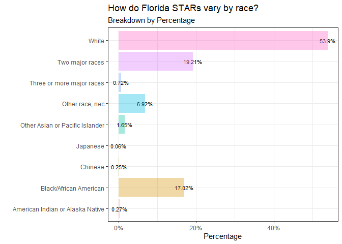
To further contextualize what I found here: 55.08% of all workers in Florida are STARs, this comes to 5154193 people.
White workers have the most presence among STARs at 53%, “two major races” came in at 19.21%, “three or more major races” reported .72%, other races are at 6.92%, while Asian/Pacific Islanders show 1.65%. The races/ethnicities reporting the least are American Indian/Alaskan Natives at .27%, Chinese at .25%, while Japanese workers have the least presence at .06%.
## Florida STAR Worker Breakdown by Location

#Table Data
fig2 <- workersdata %>%
  filter(STAR == "Yes") %>%
  group_by(location) %>%
  summarise(total = sum(person_weights)) %>%
  bind_rows(summarise(.,
                      across(where(is.numeric), sum),
                      across(where(is.character), ~"Total"))) %>% tibble()

print(fig2)
## # A tibble: 19 × 2
##    location                                 total
##    <chr>                                    <dbl>
##  1 Cape Coral-Fort Myers                  187424.
##  2 Deltona-Daytona Beach-Ormond Beach     165086.
##  3 Gainesville                             48615.
##  4 Homosassa Springs                       31813.
##  5 Jacksonville                           385529.
##  6 Lakeland-Winter Haven                  195377.
##  7 Miami-Fort Lauderdale-West Palm Beach 1457097.
##  8 Naples-Immokalee-Marco Island           75930.
##  9 North Port-Sarasota-Bradenton          196109.
## 10 Ocala                                   92208.
## 11 Orlando-Kissimmee-Sanford              656404.
## 12 Palm Bay-Melbourne-Titusville          152315.
## 13 Pensacola-Ferry Pass-Brent             125903.
## 14 Port St. Lucie                         120012.
## 15 Punta Gorda                             43676.
## 16 Sebastian-Vero Beach                    31843.
## 17 Tampa-St. Petersburg-Clearwater        766244.
## 18 <NA>                                   422608.
## 19 Total                                 5154193.
fig2 %>%
  kable() %>%
  kable_material(c("striped", "hover")) %>%
  kable_styling(bootstrap_options = c("striped", "hover", "condensed", font_size = 4)) %>%
  save_kable(file = "fig2.png")

#Plot
workersdata %>%
group_by(location, race, person_weights) %>%
  filter(STAR == "Yes") %>%
  summarise(pop_sum = sum(person_weights), label = round(pop_sum, 2)) %>%
ggplot(aes(x = pop_sum, y = location, fill = race)) +
  geom_col(alpha = .5) +
  labs(title = "Where do STARs mostly reside in Florida?",
       subtitle = "Breakdown by Metropolitan Area", x = "n", y = "", fill = "Race") +
  theme_bw() +
  theme(legend.position = "bottom")
## `summarise()` has grouped output by 'location', 'race'. You can override using the `.groups` argument.
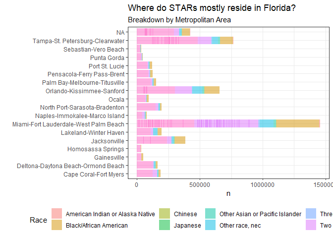
Notably, the Miami/Ft. Lauderdale/West Palm Beach metropolitan area has the most STARs at 1,457,087 workers, whereas Homosassa Springs has the least at 31813. The plots I generate later show more nuanced information, but understandably, the most diverse cultural centers in Florida have the highest concentration of STARs.
The Broward/Dade County metropolitian area has the highest concentration of immigrant workers and workers who are People of Color generally, with Hillsborogh/Pinellas, Duval and Orange/Seminole/Osceola counties not too far behind. All of these hubs house major universitiy with major arterial highways interconnected within them.
#Lookup Tables for verifying information

## Employment
employment_tbl <- workersdata %>%
  group_by(education, occupation, empstat) %>%
  filter(STAR == "Yes") %>%
  tally() %>%
  ungroup()

## Industry
industry_tbl <- workersdata %>%
  group_by(industry, occupation) %>%
  filter(STAR == "Yes") %>%
  tally() %>%
  arrange(desc(n)) %>%
  ungroup()

## Occupation
occ_tbl <- workersdata %>%
  group_by(occupation) %>%
  filter(STAR == "Yes") %>%
  tally() %>%
  arrange(desc(n)) %>%
  ungroup()

##Tables for different occupational groups
hr_workers <- workersdata %>%
  group_by(occupation, industry, education, hourly_wage, empstat, classwkrd) %>%
  filter(STAR == 'Yes',
        occupation == 'Human resources assistants, except payroll and timekeeping' |
         occupation == 'Human resources managers' |
         occupation == 'Human resources workers') %>%
 summarise(annual_wage = incearn) %>%
  arrange(desc(classwkrd))

##For averaging wages
hr_workers2 <- workersdata %>%
  group_by(occupation, education, classwkrd) %>%
  filter(STAR == 'Yes',
    occupation == 'Human resources assistants, except payroll and timekeeping' |
    occupation == 'Human resources managers' |
    occupation == 'Human resources workers') %>%
  summarise(annual_wage = incearn, mean_wage = round(mean(hourly_wage),2)) %>%
  arrange(desc(classwkrd))

## Payroll workers
payroll_timekeep <- workersdata %>%
  group_by(occupation, industry, education, hourly_wage, empstat, classwkrd) %>%
  filter(STAR == 'Yes',
         occupation == 'Payroll and timekeeping clerks') %>%
  summarise(annual_wage = incearn) %>%
  arrange(desc(classwkrd))

## Training and Devleopment workers
td_workers <- workersdata %>%
  group_by(occupation, industry, education, hourly_wage, empstat, classwkrd) %>%
  filter(STAR == 'Yes', occupation == 'Training and development managers' |
           occupation == 'Training and development specialists') %>%
  summarise(annual_wage = incearn) %>%
  arrange(desc(classwkrd))

## Compensation workers
comp_managers <- workersdata %>%
  group_by(occupation, classwkrd, education, industry) %>%
  filter(STAR == 'Yes', empstat == "Employed",
        occupation == 'Compensation and benefits managers' |
      occupation == 'Compensation, benefits, and job analysis specialists') %>%
  summarise(annual_wage = incearn) %>%
  arrange(desc(classwkrd))
Running the above code isn’t needed for this per say, but running them will condense the data into more digestible tables that can be used to find interesting insights into the STAR population, while providing a lot of context.
Some insights
For example, according to the US Bureau of Labor Statistics, HR Specialists as well as Training and Development Specialists have the most accessibility for STARs—Human Resources Specialists stand at 782,800 open roles at an 8% increase in hiring over the next ten years.
This tracks according to the data, among the STARs, they are the most frequented job titles across education groups in Florida with 243 workers—tied with ‘other office and administrative support workers.’
The top 5 industries with the most HR workers are in Employment services, Management (scientific, and technical consulting), Construction, Nursing care, and Banking. HR managers also share Construction as their leading industry with HR Assistants. Overall, construction businesses offer a viable means of mobility for STAR workers, and should targeted in Florida, along with Management services, Employment services and Banking.
HR Assistants fare well in Construction, libraries, schools, employment services and other executive and legislative bodies as far as industries go. Opportunities exists for workers with GEDs to gain roles as HR, primarily through on-the-job training, upskilling them internally via routes such as certification (via the SHRM, and other certs). Even without upskilling, HR Assistants stand to make $23.55 on average in compensation.
Compensation specialists command a good wage with only a High School Diploma. They also have good diversity among the industries they work in.
Payroll and Timekeeping Clerks command good coverage among STARs with High School Diplomas and 1+ years of college credit, no degree; with an average hourly rate of $23.76/hour.
P&T Clerks also have good coverage among the industries they are in, but they especially have good coverage in Justice and Public Order, outpatient care, schools, accounting firms and construction.
Training and Development personnel hold the highest paying positions in their job titles among those with only High School Diplomas or GEDs. They all hold positions in Construction and Business support services. T&D Specialists and Managers have a good path to mobility for those with only High School Diplomas/GEDs at a mean wage of $48.16/hour. …
#Write .csvs of tables for viewing and reference

list <- list(comp_managers=comp_managers, industry_tbl=industry_tbl,
             td_workers=td_workers, occ_tbl=occ_tbl,
             employment_tbl=employment_tbl, hr_workers=hr_workers,
             hr_workers2=hr_workers2, payroll_timekeep=payroll_timekeep,
             workersdata=workersdata)
for(i in names(list)){
  write.csv(list[[i]], paste0(i,".csv"))
}
Here I wrote the tables I made into separate .csvs. I recommend doing this if you want to further visualize the data in other platforms such as Tableau and PowerBI; or God forbid, Excel shudders.
Conclusion
This really illuminated a large base of workers in the United States, for me, a layperson who just found out about STARs. We always knew they existed, they were people without college degrees that graduated High School or obtained a GED. Its very important to see the push going on within insitiutions for these populations, due to the efforts underway that grant opportunties to demographics who are often STARs.
People who were typically passed over for people with college degrees are seeing more and more acceptance in higher-tier roles in orgranizations. These people are usually PoC, the disadvantaged and the disabled. Thanks to think-tanks and non-profits such as Opportuntiy@Work and Tear the Paper Ceiling, gaining employment that enable socioeconomic mobility is much further within reach.
Thank you for reading.