ETL using Rental Store Data? An excursion with SQL and Python
Introduction
Hello! I made this script to demonstrate what an ETL process looks like using my local PostgreSQL database, Python, some SQL and a schema with sample data from a DVD rental store. I’d say this is a look into days gone by with what used to be the main form of media in the world.
Otherwise, this is still a work in progress, so anyone looking at this, expect this to see some more polish in the future regarding the code and visualizations. There’s also a bunch of code, so please bear with me and as always, thanks!
…
Setup
Import libaries
import psycopg2
import pandas as pd
import numpy as np
import matplotlib.pyplot as plt
import seaborn as sns
from sqlalchemy import create_engine
Establish a connection with the database
connection = psycopg2.connect(
    host="localhost",
    database="dvdrental",
    user="postgres",
    password="localhost"
)
Extracting the Data
Query the database using SQL and read into a Pandas dataframe:
query = "WITH rental_data as (
                SELECT concat(first_name, ' ', last_name) as name,
                CASE WHEN active = 1 THEN 'Active' ELSE 'Inactive' END AS active,
                email, address, city, country, phone, rental_date, return_date,
                amount, rental_duration, rental_rate, replacement_cost, title as film_title,
                release_year, length as length_mins, rating, name as language
                    FROM rental as rent
                        JOIN customer as cust on cust.customer_id = rent.customer_id
                        JOIN inventory as items on items.inventory_id = rent.inventory_id
                        JOIN film on film.film_id = items.film_id
                        JOIN payment as pay on pay.rental_id = rent.rental_id
                        JOIN address as addy on addy.address_id = cust.address_id
                        JOIN city on city.city_id = addy.city_id
                        JOIN country on country.country_id = city.country_id
                        JOIN language on language.language_id = film.language_id
                        )
        SELECT *
        FROM rental_data
        WHERE (active = 'Active' AND country = 'United States');"

# Call to turn raw SQL into a Pandas Dataframe
df = pd.read_sql(query, connection)
…
Transforming
I’ll check for NAs and list the columns I’m working with for any inconsistencies
df.count()
Then, I’ll use a string replace call to make the domains something less lame..
# Replace email string
df['email'] = df['email'].str.replace("sakilacustomer.org", "live.com")
Some exploratory calls:
Who rented R rated movies?
R_Renters = df[df['rating'].str.contains("R")]['name'].unique()
names_df = pd.DataFrame(R_Renters, columns=['name'])
print(names_df)
Which movie was most rented?
df['film_title'].value_counts()
…
Next, I want to format some of the columns numerically so that I can use that data to make some charts. So to start with, I’ll get the means of the columns of interest so that I can see what some of that data looks like.
# Means for numeric columns
dfmeans = pd.DataFrame(df.loc[:,['length_mins', 'amount', 'rental_duration', 'rental_rate', 'replacement_cost']]
                         .mean()
                         )

dfmeans.columns =['means']
Now, I’m going to use group by, along with an agg (aggregation) call that mirrors the same functionality in R-dpylr’s summarise
# Summarise the above cell, but for the other columns in the dataset, and then assign it to an object

summarized = df.groupby('name').agg(
    mean_length=('length_mins', 'mean'),
    mean_rental_duration=('rental_duration', 'mean'),
    mean_rental_rate=('rental_rate', 'mean'),
    replace_cost_mean=('replacement_cost', 'mean'),
    num_person_rented_film=('name', 'count'),
    sum_amount=('amount', 'sum')
).reset_index()

emails = df['email'].unique()
sorted_emails = np.sort(emails)
emails_df = pd.DataFrame(sorted_emails, columns=['email'])
Next, I’ll do a concat call to merge the names and emails with the numbers in the data so that we have people we can attribute the numbers to:
#Merge Data
summarized = pd.concat([summarized, emails_df], axis=1, ignore_index=True)

#Rename columns
summarized = summarized[[0, 7, 1, 2, 3, 4, 5, 6]].rename(columns={
    0: 'name',
    7: 'email',
    1: 'mean_length',
    2: 'mean_rental_duration',
    3: 'mean_rental_rate',
    4: 'replace_cost_mean',
    5: 'num_person_rented_film',
    6: 'sum_amount'
})

#Print and check for errors
print(summarized.head)
…
Some Visuals
With the needed data summarized, I’m going to make a few plots to display what the data looks like based on some questions I had and previous observations.
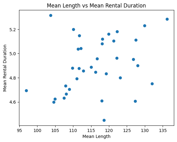
Scatter Plot:
plt.scatter(summarized['mean_length'], summarized['mean_rental_duration'])
plt.title('Mean Length vs Mean Rental Duration')
plt.xlabel('Mean Length')
plt.ylabel('Mean Rental Duration')
plt.show()
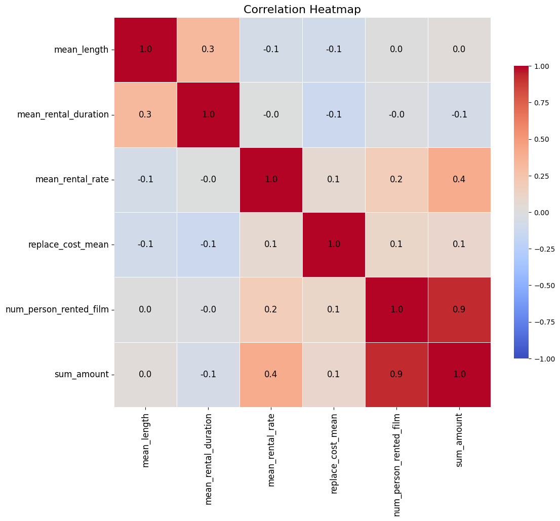
Heatmap:
# Round numbers
summarized.iloc[:, [2,3,4,5,6,7]] = summarized.iloc[:, [2,3,4,5,6,7]].round(1)

data = summarized[['mean_length', 'mean_rental_duration', 'mean_rental_rate',
                  'replace_cost_mean', 'num_person_rented_film', 'sum_amount']]

# Enhanced Heatmap
plt.figure(figsize=(12, 10))
sns.heatmap(data.corr(), annot=True, cmap='coolwarm', fmt=".1f",
            linewidths=0.5, linecolor='white', cbar_kws={"shrink": 0.75},
            annot_kws={"size": 12, "color": 'black'}, vmin=-1, vmax=1)

# Adjust the size of annotations for better readability
plt.xticks(fontsize=12)
plt.yticks(fontsize=12)
plt.title('Correlation Heatmap', fontsize=16)
plt.show()
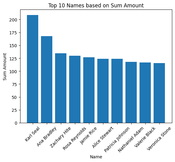
Bar Chart:
top_10 = summarized.nlargest(10, 'sum_amount')
plt.bar(top_10['name'], top_10['sum_amount'])
plt.title('Top 10 Names based on Sum Amount')
plt.xlabel('Name')
plt.ylabel('Sum Amount')
plt.xticks(rotation=45)
plt.show()
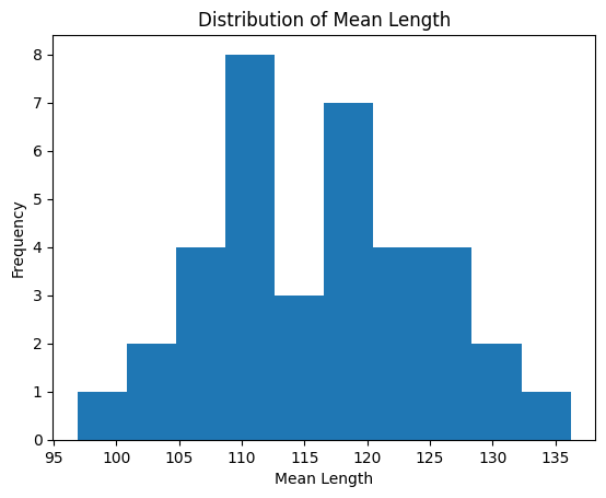
Histogram:
plt.hist(summarized['mean_length'])
plt.title('Distribution of Mean Length')
plt.xlabel('Mean Length')
plt.ylabel('Frequency')
plt.show()
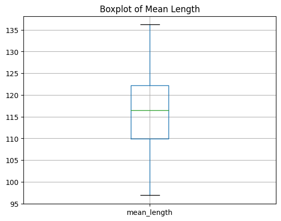
Box Plot:
summarized.boxplot(column='mean_length')
plt.title('Boxplot of Mean Length')
plt.show()
…
Loading…
Lastly, now that the visualizations are out of the way, I’m going to load the dataframes that I sourced from the original tables in my SQL database, back into that same database as different tables using the SQLAlchemy library.
Create a temporary table in PostgreSQL from the DataFrame:
engine = create_engine('postgresql+psycopg2://postgres:localhost@localhost:5432/dvdrental')
Create the tables in the dvdrental database using the existing dataframes with transformed data
df.to_sql('rental_data', engine, if_exists='replace', index = False)
summarized.to_sql('rental_temp', engine, if_exists='replace', index = False)

#Close connection:
connection.close()
Outro
In short, that was ETL in a nutshell using Python! Thank you for reading.