The Strongest of the Pocket Monsters!
This is probably the nerdiest thing you’ll ever read about Pokémon.
The beauty of this game is that fundamentally, it’s one of numbers. A bevy of formulas and calculations go into every nuance of what happens in-game. From stat modifiers, critical hits, how much damage each move does (which takes into account many variables based on stats) and even held items and their effects.
It’s what makes it such a rich game, with a simple and great lore (especially for a game made for children!).
As an avid player of the Pokémon franchise of games since childhood. I pondered: “what could I do to show off my skill in a domain that I could really sink my teeth into and relate with data-wise for this portfolio piece?”.
Having played through the Gen 2 games (think Gold, Silver and Crystal)-I wanted to do a project that analyzed trends on the Pokémon in my storage boxes.
As I journeyed around the Johto and Kanto regions, even back in the early days. I became entrenched in a never-ending journey.
Starting the EDA process
Before anything, make sure your working directory is set where you want to store all of your project’s data.
You can do that with these functions:
getwd() #Tells us where your working directory currently is

and..

setwd() # Tells R to set your working directory to a specific path
Then, for setup, we’ll need to run the needed libraries and turn off scientific notion.
library(tidyverse)
## ── Attaching packages ─────────────────────────────────────── tidyverse 1.3.2 ──
## ✔ ggplot2 3.4.0      ✔ purrr   0.3.5
## ✔ tibble  3.1.8      ✔ dplyr   1.0.10
## ✔ tidyr   1.2.1      ✔ stringr 1.4.1
## ✔ readr   2.1.3      ✔ forcats 0.5.2
## ── Conflicts ────────────────────────────────────────── tidyverse_conflicts() ──
## ✖ dplyr::filter() masks stats::filter()
## ✖ dplyr::lag()    masks stats::lag()
options(scipen = 99)
I’ll assign the .csv of my Pokémon Crystal box data to its own data set…
CrystalBox <- read.csv(file = "Data/CrystalBoxData.csv",
                       stringsAsFactors = FALSE)

# If you want, and I recommend this, use the code below to get rid of row names,
# CrystalBox$X <- NULL
…we can then look at the data using these functions:
# Look at the entire data set
View(CrystalBox)

# Look at the first few rows and their columns
head(CrystalBox)

# This gives quick summary statistics for each column in the data
summary(CrystalBox)
The code below allows us to view the class for each column in the data set, and I’ll do so for the first 10 columns.
This should give us an idea of what we’re working with, as each class of variable comes with its own set of rules.
str(CrystalBox[,1:6])
## 'data.frame':    95 obs. of  6 variables:
##  $ Sprite  : logi  NA NA NA NA NA NA ...
##  $ Position: chr  "BOX1:01" "BOX1:02" "BOX1:03" "BOX1:04" ...
##  $ Nickname: chr  "LUGIA" "SCIZOR" "MILTANK" "ABRA" ...
##  $ Species : chr  "Lugia" "Scizor" "Miltank" "Abra" ...
##  $ Nature  : chr  "Hardy" "Hardy" "Hardy" "Hardy" ...
##  $ Gender  : chr  "-" "M" "F" "M" ...
The .csv that the data was sourced from does not include types for the various assortments of Pokémon listed, so it would serve well to include them, as those columns will helps us answer many interesting questions when analyzing the data. I’ve further elaborated on the need for this a little ways down.
CrystalBox$Type1 <- NA
CrystalBox$Type2 <- NA
Next, we’ll select specific columns and then rewrite into a new data set. Some of the columns in the original data set aren’t even applicable to the way some of the mechanics in generation 2 Pokémon games work. That, or they’re just not useful. So for the purpose of this script and analysis they can be removed.
I’ll subset the needed rows using this script in dpylr:
CrystalBox <-
  CrystalBox %>%
  select(Species, Gender, HP_Type, Type1, Type2, Move1, Move2, Move3, Move4,
         HeldItem, EXP, Level, HP, ATK, DEF, SPA, SPD, SPE,
         MetLoc, MetLevel, OT, HP_IV, ATK_IV, DEF_IV, SPD_IV,
         SPE_IV, HP_EV, ATK_EV, DEF_EV, SPA_EV, SPD_EV, SPE_EV,
         IsNicknamed, IsShiny)
Once everything is completed, for this part, it’s time to write this into a .csv!
We’ll now view the changed dataet, as you can see, its cut from 90 rows to 32
View(CrystalBox)
Above, I have created two new columns; as some Pokémon have two types.
Now you can either choose to export the current .csv to Excel and edit the data manually, or you use ’c(“Psychic”, “Bug”, etc.) to enter the types manually. However, for the 95 rows of different Pokémon available, doing that will take some time.
So instead, I am using write.csv() to edit this offsite on Excel using the following functions below.
It’s important to use row.names = FALSE, because when importing the edited dataset, an unwanted column usually called “X” will appear as a placeholder. While it’s simple to remove in the console, just do this step instead.
write.csv(x = CrystalBox,
          "Data/CrystalBoxData3.csv",
          row.names = FALSE)
EDA may seem boring to many I’m sure, but it’s important to always do this when encountering a new dataset. Just to see what possible outliers or incongruities can exist in the data, before actually working with it. Plus, doing this step first and foremost can save everyone time later if done correctly.
Digging a little deeper
Now that we have looked at our data, cleaned it, doused it in Pine-Sol and gave it a good scrub. We’ll reload tidyverse and take a look at some sample questions that we can use to answer some problems with our data, to gain insights into things.
library(tidyverse)
library(knitr)
# Import data
CrystalBox <- read.csv(file = "Data/CrystalBoxData3.csv",
                       stringsAsFactors = FALSE)
What does the view from the top look like?
Lets run a summary to glean some insights.
| Species | Gender | Type1 | Type2 | Move1 | Move2 | Move3 | Move4 | EXP | Level | HeldItem |
|---|---|---|---|---|---|---|---|---|---|---|
| Lugia | - | Psychic | Flying | Aeroblast | Recover | Safeguard | Toxic | 1250000 | 100 | Leftovers |
| Scizor | M | Bug | Steel | Swords Dance | Hidden Power | Agility | Baton Pass | 125000 | 50 | Gold Berry |
| Miltank | F | Normal | NA | Body Slam | Rollout | Defense Curl | Milk Drink | 156250 | 50 | King’s Rock |
| Abra | M | Psychic | NA | Teleport | (None) | (None) | (None) | 560 | 10 | (None) |
| Granbull | M | Normal | NA | Curse | Shadow Ball | Return | Hidden Power | 100000 | 50 | TwistedSpoon |
| Ditto | - | Normal | NA | Transform | (None) | (None) | (None) | 1000 | 10 | (None) |
Columns 1-8 are very interesting, especially the gender and type columns, so I’ll run table() to investigate further
##
##  -  F  M
## 13 18 64
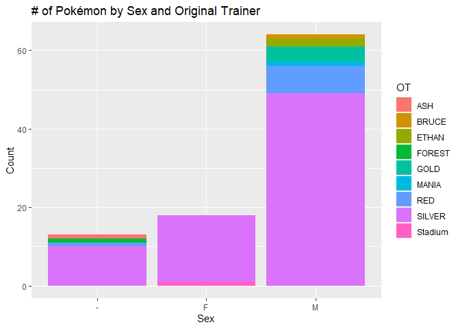
According to the data, I have 64 male Pokémon, 18 female Pokémon and 13 genderless. As an aside, there exists a programming quirk in Gen 2 where stats have a bias towards male Pokémon.
So next, let’s take a better look at the types of Pokémon we have.
## # A tibble: 95 × 3
##    Species  Type1   Type2
##    <chr>    <chr>   <chr>
##  1 Lugia    Psychic Flying
##  2 Scizor   Bug     Steel
##  3 Miltank  Normal  <NA>
##  4 Abra     Psychic <NA>
##  5 Granbull Normal  <NA>
##  6 Ditto    Normal  <NA>
##  7 Metapod  Bug     <NA>
##  8 Kakuna   Bug     <NA>
##  9 Unown    Psychic <NA>
## 10 Vulpix   Fire    <NA>
## # … with 85 more rows
I recommend assigning the above to a different dataset to view everything in detail.
Apparently, I have an overwhelming amount of water types within my boxes at 21. As we can see here:
CrystalBox %>%
  filter(Type1 == "Water") %>%
 count(Type1)
##   Type1  n
## 1 Water 21
Most of my Pokémon that do have a second type are Flying, they’re likely to be legendary Pokémon.
Most of the Pokémon I have are only of one type it seems judging by the amount of zeros in this table, as they account for the NAs that are being reported. In fact we can run the below to make sure…
CrystalBox %>%
  filter(!complete.cases(Type1, Type2)) %>%
  pull(Species)
##  [1] "Miltank"    "Abra"       "Granbull"   "Ditto"      "Metapod"
##  [6] "Kakuna"     "Unown"      "Vulpix"     "Sandshrew"  "Ampharos"
## [11] "Snorlax"    "Sentret"    "Koffing"    "Dratini"    "Suicune"
## [16] "Furret"     "Remoraid"   "Lickitung"  "Marill"     "Persian"
## [21] "Electabuzz" "Krabby"     "Hitmonlee"  "Alakazam"   "Dragonair"
## [26] "Raikou"     "Entei"      "Sudowoodo"  "Stantler"   "Seel"
## [31] "Arcanine"   "Ursaring"   "Magmar"     "Blissey"    "Meganium"
## [36] "Typhlosion" "Machamp"    "Togepi"     "Tauros"     "Vaporeon"
## [41] "Pinsir"     "Psyduck"    "Pikachu"    "Smeargle"   "Tangela"
## [46] "Seaking"    "Mewtwo"     "Donphan"    "Feraligatr" "Umbreon"
## [51] "Espeon"
The above gives us a list of Pokémon that do not have a 2nd type, but that won’t negatively affect what we need to do with our data as it’s commonplace in Pokémon for them to only have one Type.
Lets take a look at EXP and Levels:
##       EXP              Level
##  Min.   :    100   Min.   :  5.00
##  1st Qu.:   3763   1st Qu.: 15.50
##  Median : 120500   Median : 50.00
##  Mean   : 121588   Mean   : 37.73
##  3rd Qu.: 146879   3rd Qu.: 50.00
##  Max.   :1250000   Max.   :100.00
That’s about right considering the volume of Pokémon in my boxes that are around level 50.
Lets take a look at items:
##
##       (None)  Amulet Coin  Berry Juice Berserk Gene Bitter Berry   Black Belt
##           46            1            1            3            1            1
##  Brick Piece BrightPowder  Burnt Berry     Charcoal   Focus Band   Gold Berry
##            1            1            1            1            1            2
##   Hard Stone  King's Rock    Leftovers   Light Ball    Lucky Egg   Metal Coat
##            1            1            8            1            1            1
## Metal Powder Miracle Seed MiracleBerry Mystic Water     Pink Bow  Poison Barb
##            1            3            1            3            1            2
##   Quick Claw   Sacred Ash   Scope Lens  Silver Leaf SilverPowder   Smoke Ball
##            2            1            1            1            1            2
##    Soft Sand   Thick Club TwistedSpoon
##            1            1            1
It seems as though Leftovers is the most common item among my boxed Pokémon. A lot of the sets I’ve made were purpose-built for competitive battling and other nerdiness…so that’s about right.
Stats
Now lets take a look at the Pokémon’s stats. For ease of use, I’ll use tidyverse functions.
For starters:
Which Pokémon has the highest Attack stat?
CrystalBox %>%
  filter(ATK == max(ATK)) %>%
  pull(Species)
## [1] "Ho-Oh"
This gives us Ho-Oh the Rainbow Pokémon!
Which Pokémon has the highest level?
CrystalBox %>%
  filter(Level == "100") %>%
  pull(Species)
## [1] "Lugia" "Ho-Oh" "Mewtwo"
We’re tied with Lugia, Ho-Oh and Mewtwo
Which Pokémon has the highest Stat totals among them?
CrystalBox %>% group_by(Species) %>%
  summarise(total_stats = sum(HP, ATK, DEF, SPA, SPD, SPE)) %>%
  filter(total_stats == max(total_stats))
## # A tibble: 3 × 2
##   Species total_stats
##   <chr>         <int>
## 1 Ho-Oh          2053
## 2 Lugia          2053
## 3 Mewtwo         2053
Again, we have a three way tie between Lugia, Ho-Oh and Mewtwo. All have the same base stat totals, so at maximum leveling (which is 100 and maximum StatEXP), they all have the same total stats.
However, what do “base stat totals” and “StatEXP” mean? Let’s take a look.
A Quick Explanation of “Hidden Stats”
Its important to consider the following for this next section. As a few columns in the data refer to these stats.
For example, see below:
##    Species HP_IV ATK_IV DEF_IV SPD_IV SPE_IV HP_EV ATK_EV DEF_EV SPA_EV SPD_EV
## 1    Lugia    15     15     15     15     15 65535  65535  65535  65535  65535
## 2   Scizor    15     13     13     11     15 65535  65535  65535  65535  65535
## 3  Miltank    15     15     15     15     15     0      0      0      0      0
## 4     Abra    10      7      4      6      7     0      0      0      0      0
## 5 Granbull     7     12     15     13     15 65535  65535  65535      0      0
## 6    Ditto     2      8     14      0      1     0      0      0      0      0
##   SPE_EV
## 1  65535
## 2  65535
## 3      0
## 4      0
## 5  65535
## 6      0
The way Pokémon get stronger in the Gen 1 & Gen 2 games is as they battle different Pokémon, their base stats get added to the winning Pokémon’s total individual stats. This is called StatEXP.
This is referred to as “EVs” in the data, meaning “Effort Values” to maintain compatibility with newer games, Gen 3 and up.
So for example, if my Pikachu knocks out a wild Raticate-then all of Raticate’s base stats are added to Pikachu’s StatEXP totals, making him stronger.
All Pokémon can max out each individual stat for a total of 393210, 65535 for each stat.
Needless to say, a lot of grinding is needed for getting the ideal stats you want and decisively winning in battle.
What Accounts for Power?
Now that we have some context, let’s to try and determine the best team I can come up with by seeing which Pokémon acquired the most StatEXP.
First, lets total up the EXP gained by each Pokémon…
CrystalBox$Total_EV <- rowSums(CrystalBox[,26:31])
…then we’ll assign it to it’s own column in our main dataset
Let’s quickly resort everything, as the data reads better this way in my opinion.
CrystalBox <- CrystalBox %>% select(1:31, 34, 32:33)
Then run the line below and it’ll give you…
CrystalBox %>%
  filter(Total_EV == "393210") %>%
  pull(Species)
##  [1] "Lugia"      "Scizor"     "Gyarados"   "Ho-Oh"      "Zapdos"
##  [6] "Forretress" "Raikou"     "Entei"      "Arcanine"   "Ursaring"
## [11] "Steelix"    "Machamp"    "Poliwrath"  "Vaporeon"   "Aerodactyl"
## [16] "Rhydon"     "Charizard"  "Nidoking"   "Tyranitar"  "Smeargle"
## [21] "Moltres"    "Tentacruel" "Mewtwo"     "Gengar"     "Donphan"
## [26] "Feraligatr" "Umbreon"    "Espeon"
…the 28 different Pokémon that share the distinction of being trained to their utmost limits!
I can also run the code below to get a more nuanced list of Pokémon that fit this critera using base R. I certainly recommend making this into it’s own dataset to view everything, plus we’ll need to use it a bit later.
StrongestMons <- CrystalBox[which(CrystalBox$Total_EV == max(CrystalBox$Total_EV)), ]
| Species | Gender | Type1 | Type2 | Move1 | Move2 | Move3 | Move4 | EXP | Level | HeldItem | HP | ATK | DEF | SPA | SPD | SPE | MetLoc | MetLevel | OT | HP_IV | ATK_IV | DEF_IV | SPD_IV | SPE_IV | HP_EV | ATK_EV | DEF_EV | SPA_EV | SPD_EV | SPE_EV | Total_EV | IsNicknamed | IsShiny | |
|---|---|---|---|---|---|---|---|---|---|---|---|---|---|---|---|---|---|---|---|---|---|---|---|---|---|---|---|---|---|---|---|---|---|---|
| 1 | Lugia | - | Psychic | Flying | Aeroblast | Recover | Safeguard | Toxic | 1250000 | 100 | Leftovers | 415 | 278 | 358 | 278 | 406 | 318 | Whirl Islands | 60 | SILVER | 15 | 15 | 15 | 15 | 15 | 65535 | 65535 | 65535 | 65535 | 65535 | 65535 | 393210 | FALSE | FALSE |
| 2 | Scizor | M | Bug | Steel | Swords Dance | Hidden Power | Agility | Baton Pass | 125000 | 50 | Gold Berry | 176 | 179 | 149 | 102 | 127 | 116 | National Park | 14 | SILVER | 15 | 13 | 13 | 11 | 15 | 65535 | 65535 | 65535 | 65535 | 65535 | 65535 | 393210 | FALSE | FALSE |
| 12 | Gyarados | M | Water | Flying | Rain Dance | Hidden Power | Thunder | Hydro Pump | 156250 | 50 | Leftovers | 193 | 173 | 128 | 111 | 151 | 132 | Lake of Rage | 40 | SILVER | 7 | 12 | 13 | 15 | 15 | 65535 | 65535 | 65535 | 65535 | 65535 | 65535 | 393210 | TRUE | FALSE |
| 16 | Ho-Oh | - | Fire | Flying | Solar Beam | Recover | Sacred Fire | Sunny Day | 1250000 | 100 | Sacred Ash | 415 | 358 | 278 | 318 | 406 | 278 | Tin Tower | 60 | SILVER | 15 | 15 | 15 | 15 | 15 | 65535 | 65535 | 65535 | 65535 | 65535 | 65535 | 393210 | FALSE | FALSE |
| 29 | Zapdos | - | Electric | Flying | Thunderbolt | Drill Peck | Thunder Wave | Reflect | 156250 | 50 | BrightPowder | 196 | 139 | 136 | 176 | 141 | 151 | (None) | 0 | RED | 15 | 13 | 15 | 15 | 15 | 65535 | 65535 | 65535 | 65535 | 65535 | 65535 | 393210 | TRUE | FALSE |
| 30 | Forretress | M | Bug | Steel | Spikes | Rapid Spin | Toxic | Giga Drain | 125000 | 50 | Leftovers | 181 | 141 | 191 | 111 | 111 | 91 | Route 36 | 10 | GOLD | 15 | 15 | 15 | 15 | 15 | 65535 | 65535 | 65535 | 65535 | 65535 | 65535 | 393210 | FALSE | FALSE |
As you can see above, all the Pokémon listed have Total Evs at 393210; making them obscenely powerful.
So my group seems to be super strong, and this is very indicative that I put in the time into grinding, which I’m low key ashamed of.
Needless to say, when I want to win a battle; I’ll need to send out a combination of those 28 Pokémon from Crystal to crush my opponent.
Ash Ketchum and PKMN Trainer Red never stood a chance.
Strongest of the Strong
Now we’re going to find the answer to the question: “which team can I put together of these 28 that can be considered the strongest based on our data?”
Let’s start here:
StrongestMons$StatTotals <- rowSums(StrongestMons[,12:17])

CrystalBox$StatTotals <- rowSums(CrystalBox[,12:17])
We’ll also do the same for our main dataset, as the visualizations coming up next will need to reference this specific column
This gives us 2053 stats for each observation, which indicates that all three Pokémon have reached the same limits, however, before we get to the meat and potatos of things. We’ll take a brief look at how stats are calculated.
A quick primer on Base Stats (BST)
These formulas below calculate base stats:
For Hit Points: $Stat = floor((2 * B + I + E) * L / 100 + L + 10)$
For all Stats: $floor(floor((2 * B + I + E) * L / 100 + 5) * N)$
For Gen 2 Effort Values: $E = floor(min(255, ceiling(sqrt(StatEXP))) / 4)$
Legend:
B = Base Stat
I = Individual Values, Gen 1 & 2 only go up to 15, so multiply 15 by 2
E = Effort Values, see above for StatEXP explanation, the formula used here is different for the older system’s methods
L = Level
N = Nature, which doesn’t exist in Gens 1 & 2, so N is = 1
The most important thing to note about what’s listed above is that it gives context for why certain Pokémon excel in certain facets of battle than others.
When it comes to Base Stats (otherwise known as BST), another awesome eccentricity of Pokémon is that every individual creature has strengths that can potentially put them head and shoulders above the rest. Especially when it comes to fulfilling certain roles on a team.
This all builds up to answer the question: “Among all of my boxed Pokémon, which are the strongest?”
Well, three Pokémon at level 100 qualify, as all their stats total to
- Its safe to say that Lugia, Ho-Oh and Mewtwo are all tied for 1st because in Gens 1 & 2; no other Pokémon have higher than 680 for their total base stats!
Now lets see what measures up to the literal gods of Pocket Monsters!
The Definitive Answer
Since we’ve already made our ‘StatTotals’ column above, now we’re going to use that to choose the six strongest Pokémon we’ve found and put them into one team:
StrongestTeam <- StrongestMons %>%
  filter(StatTotals < 2053) %>%
  top_n(6,StatTotals)
That gives us, Zapdos, Raikou, Entei, Arcanine, Tyranitar and Moltres. However, something isn’t right…4/6 of those Pokémon are indeed legendary and while not as godly, are still in a different league to that of our mortal Pocket Monsters.
So let’s do something about that.
StrongestMons$IsLegendary <- c("Yes", "No", "No", "Yes", "Yes", "No",
                                      "Yes", "Yes", "No","No", "No", "No", "No",
                                      "No", "No", "No", "No", "No", "No", "No",
                                      "Yes", "No", "Yes", "No", "No", "No",
                                      "No", "No")
The above line will tell us if a particular Pokémon is “legendary” or not as Legendary Pokémon tend to have base stat totals above 580 which are factored in the StatTotal column I made earlier
So therefore, what if I wanted to select a team of the six strongest regular Pokémon I have with a StatTotal that nearly equals that of my legendaries?
StrongestTeam <- StrongestMons %>%
  distinct(StatTotals, .keep_all = "True") %>%
  filter(StatTotals < 2053, IsLegendary == "No") %>%
    top_n(6 , StatTotals)
This will give you an idea:
## [[1]]
## [1] "Gyarados"   "Arcanine"   "Charizard"  "Tyranitar"  "Feraligatr"
## [6] "Umbreon"
When all the calculations are said and done. It appears that Gyarados, Arcanine, Charizard, Tyranitar, Feraligatr, and Umbreon seem like the most viable picks, sure to win me a championship or two.
However, an important nuance to consider here when looking at my Pokémon’s levels are the levels. At level 50, my code determines that the Pokémon listed are the strongest based on the BST I’ve set in the criteria.
Levels are an important thing to distinguish in this regard, because it determines the unrealized potential of the other gained stats of each mon.
The cool thing here is that due to all of our Pokémon’s stats being maxed out, they’ll still be every bit as strong relative to their stats at Level 100, as they would be at Level 50. This doesn’t change in games even as recent as Generation 8’s.
In fact if Gen 2 had an endgame boss that wasn’t Pkmn Trainer Red (…!), I could see him using this team.
…
Example Data Visualization/assets/images/s
This section is going to outline all of the visualizations I can think of that can give further context to the data we have on hand. While also giving insight to the line of thinking needed to ascertain what visualization method is best suited for a given use case.
One variable, discrete variables
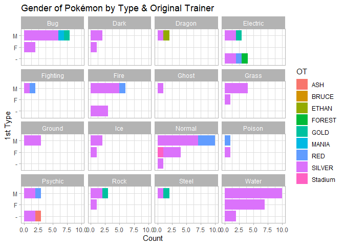
ggplot(CrystalBox, aes(y = Gender, fill = OT)) +
   geom_bar() +
   xlim(0,10) +
   xlab("Count") +
   ylab("1st Type") +
   ggtitle("Gender of Pokémon by Type & Original Trainer") +
   theme_light() +
   facet_wrap(Type1 ~ .)
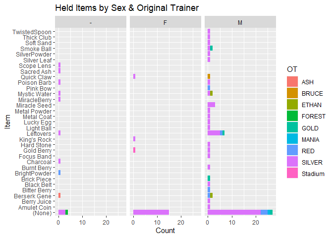
ggplot(CrystalBox, aes(y = HeldItem, fill = OT)) +
         geom_bar() +
  ggtitle("Held Items by Sex & Original Trainer") +
  xlab("Count") +
  ylab("Item") +
  facet_wrap(Gender ~ .)
ggplot(CrystalBox, aes(x = Gender, fill = OT)) +
  geom_bar() +
  ggtitle("# of Pokémon by Sex and Original Trainer") +
  xlab("Sex") +
  ylab("Count")
#One variable, continuous

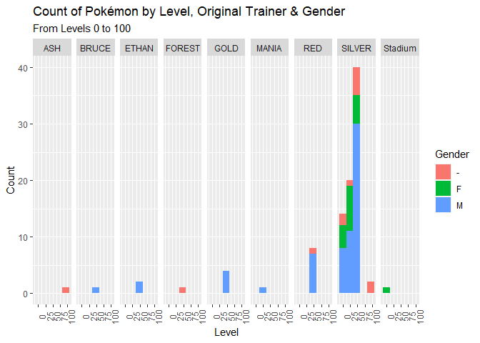
ggplot(CrystalBox, aes(x = Level, fill = Gender)) +
  geom_histogram(bins = 5, position = "stack") +
  ggtitle("Count of Pokémon by Level, Original Trainer & Gender",
          subtitle = "From Levels 0 to 100") +
  ylab("Count") +
  theme(axis.text.x = element_text(angle = 90),
        axis.text.y = element_text(angle = 0)) +
  facet_grid(cols = vars(OT))
…
Two variable plots
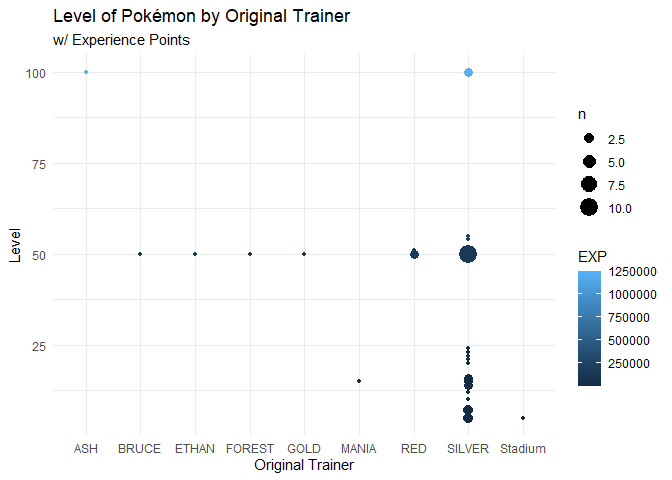
#Ver. 1
ggplot(CrystalBox, aes(x = OT, y = Level, color = EXP)) + geom_count() +
  ggtitle("Level of Pokémon by Original Trainer",
          subtitle = "w/ Experience Points") +
  xlab("Original Trainer") +
  theme_minimal()
#Ver. 2 — Using Facet Wrap
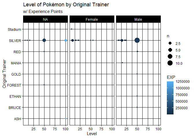
gender.labs <- c("Genderless", "Male", "Female")
names(gender.labs) <- c("Genderless", "M", "F")
ggplot(CrystalBox, aes(x = Level, y = OT, color = EXP)) + geom_count() +
  ggtitle("Level of Pokémon by Original Trainer",
          subtitle = "w/ Experience Points") +
  xlab("Level") +
  ylab("Original Trainer") +
  theme_linedraw() +
  facet_wrap(Gender ~ ., labeller = labeller(Gender = gender.labs))
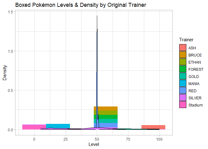
ggplot(CrystalBox, aes(x = Level, y = ..density.., fill = OT)) +
  geom_histogram(bins = 6) +
  geom_density(kernel = "gaussian") +
  ggtitle("Boxed Pokémon Levels & Density by Original Trainer") +
  scale_fill_discrete(name = "Trainer") +
  xlab("Level") +
  ylab("Density") +
  theme_light()
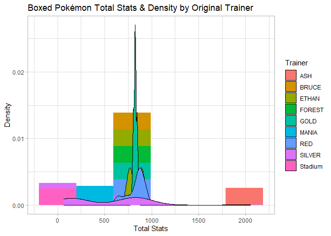
ggplot(CrystalBox, aes(x = StatTotals, y = after_stat(density), fill = OT)) +
  geom_histogram(bins = 6) +
  geom_density(kernel = "gaussian") +
  theme(axis.title.x = element_text(face = "bold",
          margin = margin(t = 0, r = 0, b = 10, l = 0)),
        axis.title.y = element_text(face = "bold",
            margin = margin(t = 0, r = 10, b = 0, l = 0))) +
  ggtitle("Boxed Pokémon Total Stats & Density by Original Trainer") +
  scale_fill_discrete(name = "Trainer") +
  xlab("Total Stats") +
  ylab("Density") +
  theme_light()
…
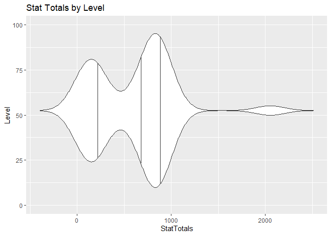
Sample violin plot, with quantiles.
ggplot(CrystalBox, aes(x = Level, y = StatTotals)) +
  geom_violin(draw_quantiles = c(0.25, 0.50, 0.75), trim = FALSE) +
  xlim(0,100) +
  ylab("StatTotals") +
  ggtitle("Stat Totals by Level") +
  coord_flip()
…
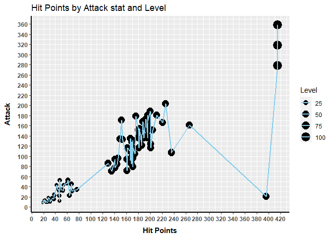
Line graphs showing correlation between Hit points and offensive stats by level
ggplot(CrystalBox, aes(x = HP, y = ATK, size = Level)) +
  geom_point() +
  geom_line(linewidth = 1, color = "sky blue") +
  xlab("Hit Points") +
  ylab("Attack") +
  scale_x_continuous(breaks = scales::pretty_breaks(n = 20)) +
  scale_y_continuous(breaks = scales::pretty_breaks(n = 15)) +
  ggtitle("Hit Points by Attack stat and Level") +
  theme(axis.text.x = element_text(face = "bold"),
        axis.text.y = element_text(face = "bold"),
        axis.title.x = element_text(face = "bold",
          margin = margin(t = 8, r = 10, b = 0, l = 0)),
        axis.title.y = element_text(face = "bold",
            margin = margin(t = 0, r = 10, b = 0, l = 0)),
        axis.line = element_line(colour = "black",
        linewidth = 1, linetype = "solid"))
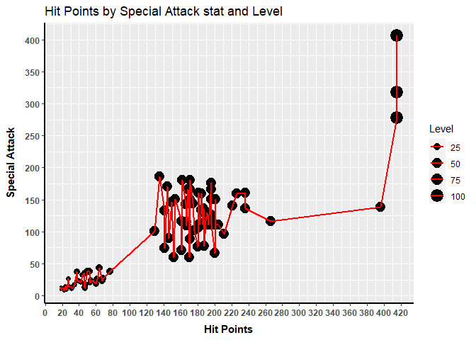
ggplot(CrystalBox, aes(x = HP, y = SPA, size = Level)) +
  geom_point() +
  geom_line(linewidth = .75, color = "red") +
  xlab("Hit Points") +
  ylab("Special Attack") +
  scale_x_continuous(breaks = scales::pretty_breaks(n = 20)) +
  scale_y_continuous(breaks = scales::pretty_breaks(n = 15)) +
  ggtitle("Hit Points by Special Attack stat and Level") +
  theme(axis.text.x = element_text(face = "bold"),
        axis.text.y = element_text(face = "bold"),
        axis.title.x =
          element_text
            (face = "bold", margin = margin(t = 8, r = 10, b = 0, l = 0)),
        axis.title.y =
          element_text
            (face = "bold", margin = margin(t = 0, r = 10, b = 0, l = 0)),
        axis.line = element_line(colour = "black",
                                 linewidth = 1, linetype = "solid"))
…
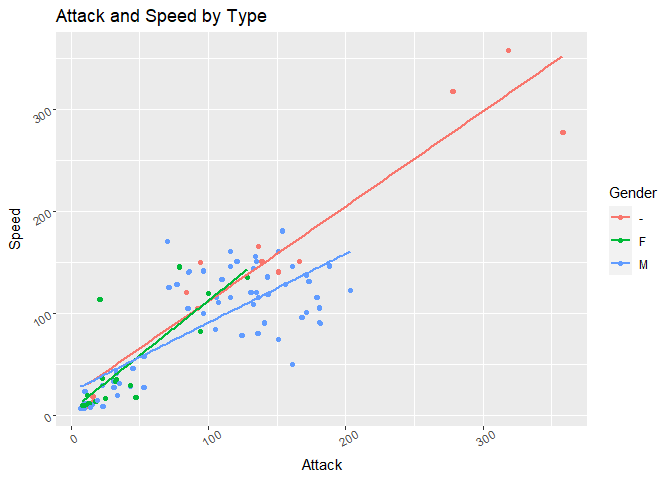
Different graphs showing correlation between offensive stats and speed
ggplot(CrystalBox, aes(x = ATK, y = SPE, color = Gender)) +
  ggtitle("Attack and Speed by Type") +
  xlab("Attack") +
  ylab("Speed") +
  theme(axis.text.x = element_text(angle = 30),
        axis.text.y = element_text(angle = 30)) +
  geom_jitter() +
  geom_point() +
  scale_fill_continuous(type = "viridis") +
  geom_smooth(method = lm, se = FALSE)
## `geom_smooth()` using formula = 'y ~ x'
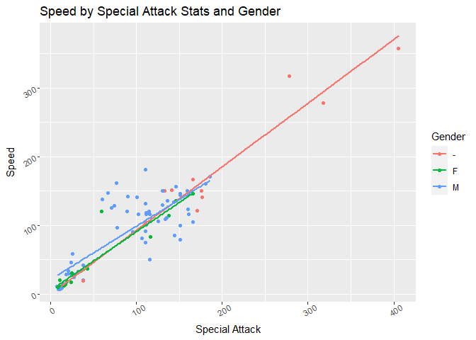
ggplot(CrystalBox, aes(x = SPA, y = SPE, color = Gender)) +
  geom_jitter() +
  xlab("Special Attack") +
  ylab("Speed") +
  ggtitle("Speed by Special Attack Stats and Gender") +
  geom_smooth(method = lm, se = FALSE) +
  theme(axis.text.x = element_text(angle = 30),
        axis.text.y = element_text(angle = 30)
  )
## `geom_smooth()` using formula = 'y ~ x'
#Attack and Speed density plot
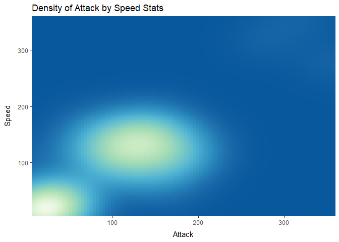
ggplot(CrystalBox, aes(x = ATK, y = SPE)) +
  ggtitle("Density of Attack by Speed Stats") +
  xlab("Attack") +
  ylab("Speed") +
  stat_density_2d(aes(fill = ..density..), geom = "raster", contour = FALSE) +
  scale_fill_distiller(palette = 4, direction = -1) +
  scale_x_continuous(expand = c(0, 0)) +
  scale_y_continuous(expand = c(0, 0)) +
  theme(
    legend.position = 'none',
    axis.title.x = element_text(margin = margin(
      t = 8,
      r = 10,
      b = 0,
      l = 0
    )),
    axis.title.y = element_text(margin = margin(
      t = 0,
      r = 10,
      b = 0,
      l = 0
    )),
  )
Heatmap
I’ll admit, making a heatmap using base R was a lot more difficult than I realized. So much has to go into properly formatting whatever you’re putting in the x axis if your data isn’t properly aggregated. If you’re looking to make more nuanced heatmaps(), I recommend heatmap2() and pheatmap().
Firstly, you have to make sure all the variables you’re putting into the heatmap are numeric, due to the design of how the chart works. So if you have variables that are non-numeric like character-based columns that you want to have accounted for, you’ll need to make counts for each instance and then coalesce them into the main data set you want to chart. I digress.
Here we go!
# Subset main dataset
CrystalBoxHM <-  subset(CrystalBox[,c(3:4,9:10,12:17,19,21:31)])

# Edit the source data set for use with the heatmap, as heatmaps can only be used with matrices containing
# numeric variables
 #Replace NAs with blank spaces for sum functions below

CrystalBoxHM[,2] <-
   replace(CrystalBoxHM$Type2,is.na(CrystalBoxHM$Type2),"")


 #Make Type columns

CrystalBoxHM2 <- unique( CrystalBoxHM[ , 1 ] )
CrystalBoxHM2 <- as.data.frame(CrystalBoxHM2)

CrystalBoxHM2$Type2 <- NA
colnames(CrystalBoxHM2) <- c("Type1", "Type2")
CrystalBoxHM2$Type2 = CrystalBoxHM2$Type1  #Run first

CrystalBoxHM2 <- CrystalBoxHM2 %>% add_row(Type1 = "Flying")
CrystalBoxHM2$Type2 = CrystalBoxHM2$Type1 #Run again

#See above, since the main data set doesn't account for Flying types in Type 1 as they're no pure Flying types in all of Pokémon.

#Make counts of Type 1 & 2 columns

CrystalBoxHM2$Type1_Count <-
   sapply(CrystalBoxHM2[,1], function(string)
     sum(string == CrystalBoxHM[,1]))

CrystalBoxHM2$Type2_Count <-
   sapply(CrystalBoxHM2[,2], function(string)
     sum(string == CrystalBoxHM[,2]))

#Edit row names for heatmap

row.names(CrystalBoxHM2) <- c("Psychic",  "Bug", "Normal", "Fire",
                                    "Ground", "Water",  "Electric",
                                    "Poison", "Dragon", "Ice", "Dark",
                                    "Fighting", "Rock", "Steel",  "Grass",
                                    "Ghost", "Flying")

#Make other columns for the matrix that the heatmap will be based on...


#Make Type counts for the other data set we subsetted originally:

CrystalBoxHM$Type1_Count <-
   sapply(CrystalBoxHM[,1], function(string)
     sum(string == CrystalBoxHM[,1]))


CrystalBoxHM$Type2_Count <-
   sapply(CrystalBoxHM[,2], function(string)
     sum(string == CrystalBoxHM[,2]))

#Splitting data, merging new datasets, summarizing and subsetting:

Type1_meanEXP <-
   CrystalBoxHM %>% group_by(Type1) %>% summarize(mean_EXP = mean(EXP))

Type1_meanEXP <-
   Type1_meanEXP %>% remove_rownames %>%
   column_to_rownames(var = "Type1") %>%  as.data.frame()

meanEXP2 <- merge(CrystalBoxHM2, Type1_meanEXP, by = 0, all = TRUE)

meanEXP2 <-
   meanEXP2 %>% remove_rownames %>%
   column_to_rownames(var = "Row.names") %>%  as.data.frame()

#Note above that we must change the row names to the types that will display in the heatmap, because remember, heatmaps can only be used with dataset that contain columns with only numeric properties. Row names are not affected by this.

#Merge and null unneeded columns

meanEXP2[,1:2] <- NULL

#New data with all the means we need

all_means <- subset(CrystalBoxHM, select = c(Type1:Type2, Level, HP:SPE))

all_means[, 10:16] <- colMeans(x = all_means[, 3:9])

all_means[, 3:9] <- NULL

#Rename rows to proper averages:

all_means <- all_means %>%
   rename(
     Level_Avg = V10,
     HP_Avg = V11,
     ATK_Avg = V12,
     DEF_Avg = V13,
     SPA_Avg = V14,
     SPD_Avg = V15,
     SPE_Avg = V16
   )

#Re-summarise all the means in our group

all_means <-
   all_means %>% group_by(Type1) %>% summarise_all(mean)

all_means[, 2] <- NULL

all_means <-
   all_means %>% remove_rownames %>% column_to_rownames(var = "Type1") %>%  as.data.frame()

#Merge everything and fix row names:

meanEXP2 <- merge(meanEXP2, all_means,  by = 0, all = TRUE)


meanEXP2 <-
   meanEXP2 %>% remove_rownames %>% column_to_rownames(var = "Row.names") %>%
   as.data.frame()

CrystalBoxHM3 <- meanEXP2 #I renamed the merged dataset to maintain consistency.
#The heatmap itself

par(cex.main = .85)

heatmap(as.matrix(x = CrystalBoxHM3), scale="col",
         margins = c(6, 6),
         Colv = NA,
         na.rm = TRUE,
         main = "Aggregations by Type",
         xlab= "Aggregates",
         ylab= "Type",
         cexCol=.75, col = cm.colors(256))
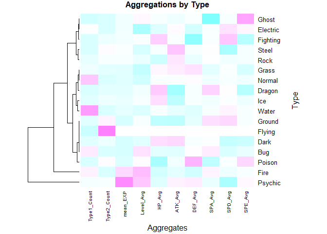
#Note how I edited the code to remove the column dendrogram from the chart.
Outro
When it comes to the intricate details of Pokémon, you’ll start to unravel many layers to a game that seems rather innocuous on the outside.
Frankly, when I started to delve deeper and deconstruct one of my all-time favorite games in this manner; it took a good amount of self-reflection. Data is certainly something I find passion in doing well, but sometimes when it comes to games—–the fun comes in the mystery that comes with discovering novel things, and joy that is found in the experience you have in the present moment.
While the fun of my childhood self playing Pokémon will always be seeped in nostalgia, through finding novel experiences via my pursuits in data and uncovering useful insights—I hope that can give me a similar feeling in my adult life.
I’ll always appreciate what Satoshi Tajiri gave me and millions of other youth worldwide.
Thank you for reading, Bruce A. Lee